Opportunities for Arbitrage in the Beijing Housing Market

Abstract

We build a novel real estate price dataset that contains a large sample (over 60,000 data points) of data from two major cities in China, Beijing and Shanghai. With machine learning techniques, we propose a series of supervised learning models to predict second-hand housing price with our dataset and demonstrate that our best model has a strong predictive power on housing price with a minimum Root Mean Square Error of 0.105 and a maximum R² of .965. Our experiments show that the size and the location of the property are overall the most important features to predict the total house price, yet feature importance may vary across different supervised learning models and different cities. The error analysis points out that our model is prone to make mistakes in certain districts. Also, the model does not perform consistently among districts within the same city. We tried to improve our model by introducing new features and adjusting the weights of samples of different districts. However, our attempt fails to improve the overall accuracy but reduces the variance of the prediction accuracies among districts.

Data

Data Collection

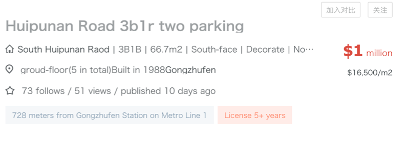
We collected the second-hand housing price information from the largest online-to-offline (O2O) real estate platform in China, Lianjia.com. Our dataset contains a collection of 21, 854 residential property records in Beijing and 38, 684 records in Shanghai. To further analyze our system’s performance against the geographical location of each property, we aggregated the longitude and latitude information to the dataset by querying Baidu API using the name information of each property’s neighborhood.

Features

Categorical	description, district, sub-district, villa, direction, decoration, has_elevator, subway_station_nearby, free_of_business_tax, free_of_all_tax, agent_haskey, floor, building_type, has_garage
Numerical	Total price (the target), longitude, latitude, area, room_number, building_age

After conversion and standardization, we obtained a 201-dimension feature vector for each property. We adopted an 80/20 training-test split on the dataset for the evaluation of our proposed models.

Methodologies

Problem Definition

After feature engineering, each property can be represented as a feature vector containing 201 features. Our goal is to train a regressor on the training set and make the sum of the squared differences between each prediction and its true value as small as possible.

Primary Models

We applied following different models as our regressor to compare their performance and exploit the feature importance out of them. They could be viewed as representatives of linear models, neural networks, tree-based methods, Bagging models and Boosting models.

• Ridge Regression
• Decision Tree
• Multi-Layer Perceptron (MLP)
• Random forest
• XGBoost

Also, we used a Linear Regression model and a K-Nearest-Neighbor (KNN) model as our baseline models. We used 5-fold cross-validation for model selection to find the optimal hyperparameter-setting for each model.

Evaluation

After tuning each model using cross-validation, we trained each of the models with the optimal hyperparameters on the entire training set and evaluated our results on the test set with root mean squared error (RMSE) and R².

Experiments and Discussion

Baselines

As for baseline analysis, we adopted Linear Regression and K-Nearest-Neighbor models.

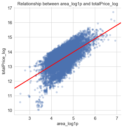
In the Linear Regression model, we regressed the dependent variable totalPrice_log on the only one independent variable area_loglp.

 In the K-Nearest-Neighbor model, we took the latitude and the longitude of the property as the feature variables and totalPrice_log as our target value.

Model Fitting

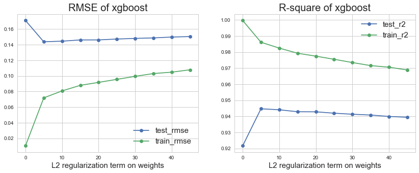
We applied grid search to tune the hyperparameters. The figure below shows the average cross-validated performance, R²and RMSE across 5 random training folds and testing folds using XGBoost. The similar process is also conducted on other models.

Feature Importance

The exploration of feature importance is considered as an essential step in our model selection, model tuning and model evaluation processes. In order to make full use of the feature importance exploration work to better our learning model, we have divided it into two phases. Within each phase, we adopted different methods to acquire feature importance ranks and analyzed the results in different lights.

Phase I Pre-training/model-fitting feature selection. In this phase and prior to any learning processes, we used random forest algorithm to fit housing price data and filtered unimportant features from the model

Phase II Post-training/model-fitting feature importance determination. After having fitted the model with data processed from phase I, we extracted among different models the feature importance so as to understand the entire research problem and reevaluate our models.

Novel Feature Analysis A special feature we include in our dataset is description-related features. Initially, we considered this group of features of great importance to our models. Surprisingly, after training our models, it turned out that all description-related features appeared zero importance to our models. As a result, we excluded these features from our final model.

Overall Results

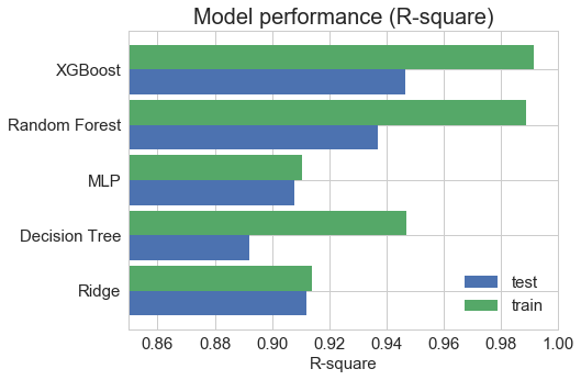
Among five models we train, we concluded that XGBoost has the best performance in terms of both R2and RMSE evaluation metric.

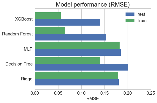
Finally, we run the model on the test set and got the following accuracy scores:

	R2	RMSE
Beijing	0.953	0.132
Shanghai	0.965	0.105

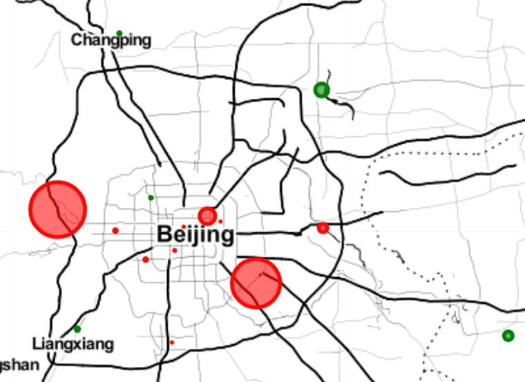
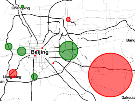
Error Analysis

When inspecting the gap between the prediction and the real value in percentage, we found out that two districts are systematically undervalued. Even though the houses in these two districts are supposed to be cheap because they are far away from the center of the city, they have their own advantages which, however, cannot be captured by our model so far. For example, the western district of Beijing is a wealthy suburb with good “ Fengshui ” (geomancy). And the district in the southeast is an economic and technological development zone, where a lot of big companies are located. As a result, the houses in these two areas should be more expensive than our model’s predictions.

The model can predict housing prices for the center of the city with an accuracy that is very close to the overall model accuracy. The reason for that is because most of the data is concentrated around the city center, as most houses there are old and takes up the largest percentage of the second-hand properties. Thus, the validity of our model applied on the data of the city center is higher than that of other districts.

According to the error analysis above, we initialized two ways to improve our model. The first method is to introduce new features. However, given the nature of our data which is scraped from the online platform, we were no longer able to add any new feature. The second method is to adjust the proportion of samples of each district to the total samples so that every district occupies an equal proportion of samples among all. By adopting such method, the performance didn’t significantly improve, but the overall district accuracy variance decreased.

Conclusion

Overall, we have performed data scraping, feature engineering and model selection with training data. Comparing different models for Beijing, we came to realize that feature importance varies according to methods adopted. From inter-district comparison within Beijing, we found out that housing prices in some districts are symmetrically undervalued or overvalued. Given the current dataset we have, our model failed to capture some latent facts that have effects on the housing price. For future improvement, we suggest collecting more data targeting at featuring some latent factors that might affect model precision when predicting housing prices in big cities.